简介

• 逻辑回归虽然顶着一个回归的名称，但是实际上做的是分类的事情。回归的一般形式可以表示为：$f(x)=wx+b$然而，分类任务的最终结果是一个确定的标签值，逻辑回归的输出范围为[-∞,+∞]，需要使用Sigmoid函数将输出Y映射为一个[0,1]之间的概率值，再根据设定的阈值分类出正样本和负样本，比如>0.5作为正样本，<0.5的作为负样本
• 逻辑回归在周志华的西瓜书中被称作对数几率函数，为了让模型去预测逼近y的衍生物，按照我的理解就是从线性推广到非线性的情况，则对数几率函数可表示为：$lny=wx+b$

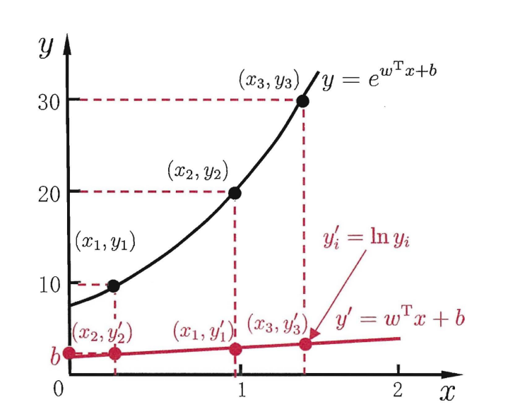
从图中可以看出，这里的对数函数起到了将线性回归模型的预测值与真实标记联系起来的作用[周志华，机器学习，p.56]

Sigmoid函数

Sigmoid函数是一个S形曲线的数学函数，在逻辑回归、人工神经网络中有着广泛的应用。Sigmoid函数的数学形式是：
$$S(t)=\frac{1}{1+e^{-t}}$$
其函数图像如下：

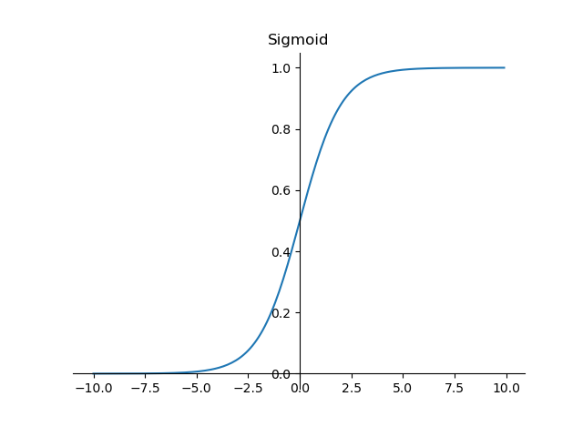
可以看出，sigmoid函数连续，光滑，严格单调，以(0,0.5)中心对称，是一个非常良好的阈值函数。

并且sigmoid函数还有一个非常好的特性，它的导函数可以用自身表示出来：
$$f^{\prime }(x)=f(x)(1-f(x))$$

import matplotlib.pyplot as plt
import numpy as np

x = np.arange(-10,10,0.1)
y = 1/(1+np.exp(-x))


fig,ax = plt.subplots()
ax.plot(x,y)
ax.set_title('Sigmoid')
ax.spines['right'].set_color('none') # 隐藏掉右边框线
ax.spines['top'].set_color('none')    # 隐藏掉左边框线
ax.xaxis.set_ticks_position('bottom')  # 设置坐标轴位置
ax.yaxis.set_ticks_position('left')  # 设置坐标轴位置
ax.spines['bottom'].set_position(('data', 0))   # 绑定坐标轴位置，data为根据数据自己判断
ax.spines['left'].set_position(('data', 0))
plt.show()

损失函数与参数更新

• 一般线性回归模型的w和b求解

线性回归试图学得f(x)=wx+b使得,f(x)无限接近y的值，如何确定w,b的值呢？关键在于衡量f(x)与y之间的差别。通常使用均方误差即square loss作为性能度量
$$\begin{array}{rl}\left(w^{\ast },b^{\ast }\right)& =\underset{(w,b)}{\mathrm{argmin}}\sum _{i=1}^m{\left(f\left(x_i\right)-y_i\right)}^2\\ & =\underset{(w,b)}{\mathrm{argmin}}\sum _{i=1}^m{\left(y_i-w{x}_i-b\right)}^2\end{array}$$
求解w和b就是使$E_{(w,b)}={\sum }_{i=1}^m{\left(y_i-w{x}_i-b\right)}^2$最小化的过程

• 逻辑回归中的w和b的求解

逻辑回归的概率损失函数可写为：
$$J(\theta )=\frac{1}{2m}\sum _{i=1}^m{\left(h_{\theta }\left(x^{(i)}\right)-y^{(i)}\right)}^2=\frac{1}{2m}\sum _{i=1}^m{\left(\frac{1}{1+e^{-{\theta }^T{x}_i-b}}-y^{(i)}\right)}^2$$
这个损失函数是非凸函数，不好优化，需要转换为最大似然函数求解w和b

逻辑回归的概率可以整合为：
$$p(y|x_i)=f(x_i{)}^{y_i}(1-f(x_i){)}^{1-y_i}$$
似然函数为：
$$L(\theta )=\prod _{i=1}^{m}P\left(y_i\mid x_i;\theta \right)=\prod _{i=1}^m{\left(h_{\theta }\left(x_i\right)\right)}^{y_i}{\left(1-h_{\theta }\left(x_i\right)\right)}^{1-y_i}$$
对数似然为：
$$l(\theta )=\log L(\theta )=\sum _{i=1}^m\left(y_i\log h_{\theta }\left(x_i\right)+\left(1-y_i\right)\log \left(1-h_{\theta }\left(x_i\right)\right)\right)$$
此处应使用梯度上升求最大值，引入$J(\theta )=-\frac{1}{m}l(\theta )$转换为梯度下降任务

对似然函数求导并化简可得：
$$\frac{\delta }{{\delta }_{{\theta }_j}}J(\theta )=-\frac{1}{m}\sum _{i=1}^m\left(y_i\frac{1}{h_{\theta }\left(x_i\right)}\frac{\delta }{{\delta }_{{\theta }_j}}{h}_{\theta }\left(x_i\right)-\left(1-{\mathrm{y}}_{\mathrm{i}}\right)\frac{1}{1-h_{\theta }\left(x_i\right)}\frac{\delta }{{\delta }_{{\theta }_j}}{h}_{\theta }\left(x_i\right)\right)$$

$$=\frac{1}{m}\sum _{i=1}^m(h_{\theta }(x_i)-y_i)x_i^j$$

Softmax

https://zhuanlan.zhihu.com/p/105722023

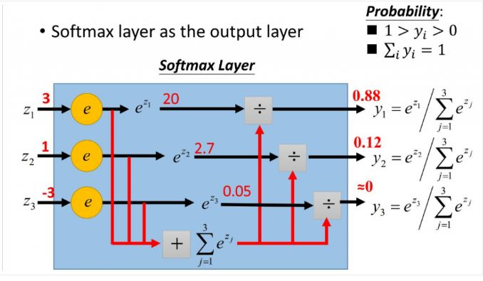
与softmax相对的是hardmax，指的是只选出其中一个最大的值。而softmax的含义就在于不再是唯一的确定某一个最大值，而是为每一个输出分类的结果都赋予一个概率值，表示属于每个类别的可能性。

softmax函数的定义：
$$\mathrm{Softmax}\left(z_i\right)=\frac{e^{z_i}}{{\sum }_{c=1}^C{e}^{z_c}}$$
其中，Zi为第i个节点的输出值，C为输出节点的个数，即分类的类别个数。

为什么使用softmax函数？

• 可以将输出的数值拉开距离

用代码试验一下。假设有三个输出节点的值(1,5,10,15)

import numpy as np
x = np.array([1,5,10,15])
y = np.exp(x) #  array([2.71828183e+00, 1.48413159e+02, 2.20264658e+04, 3.26901737e+06])
S = np.exp(x)/sum(y) # array([8.25925493e-07, 4.50940040e-05, 6.69254359e-03, 9.93261536e-01])
# 下面求不带指数形式的
Z = x/sum(x) #  array([0.03225806, 0.16129032, 0.32258065, 0.48387097])

结果显而易见，用了指数形式的将差距大的数值拉的更加大

• 第二个优点就是，ex的导函数仍是ex

求导过程可参考以下两个博客：https://www.jianshu.com/p/4670c174eb0d https://www.jianshu.com/p/6e405cecd609

求导后的结果可表示为：
$$\begin{array}{rl}& \frac{\partial L_i}{\partial W_{ij}}=\{\begin{array}{ll}\left(S_i-1\right)x_j& ,y=i\\ S_i{x}_j& ,y\ne i\end{array}\\ & \frac{\partial L_i}{\partial b_i}=\{\begin{array}{ll}\left(S_i-1\right)& ,y=i\\ S_i& ,y\ne i\end{array}\end{array}$$
其中，S为softmax函数，y为标签值。对应代码：

def L_Gra(W, b, x, y):
    """
     W,b 为当前的权重和偏置参数，x，y为样本数据和该样本对应的标签
    """
    # 初始化
    W_G = np.zeros(W.shape)
    b_G = np.zeros(b.shape)
    S = softmax(np.dot(W,x) + b)
    W_row = W.shape[0]
    W_column = W.shape[1]
    b_column = b.shape[0]

    # 对Wij和bi分别求梯度
    for i in range(W_row):
        for j in range(W_column):
            W_G[i][j] = (S[i] - 1) * x[j] if y == i else S[i] * x[j] # S: softmax函数 为什么没用到loss？求解过程中已经加入了

    for i in range(b_column):
        b_G[i] = S[i] - 1 if y == i else S[i]
    return W_G, b_G

def L_Gra(W, b, x, y):
    """
     W, b为当前的权重和偏置参数，x,y为样本数据和该样本对应的标签
    """
    #初始化
    W_G = np.zeros(W.shape)
    b_G = np.zeros(b.shape)
    S = softmax(np.dot(W,x) + b)
    W_row=W.shape[0]
    W_column=W.shape[1]
    b_column=b.shape[0]
    #对Wij和bi分别求梯度
    for i in range(W_row):
        for j in range(W_column):
            W_G[i][j]=(S[i] - 1) * x[j] if y==i else S[i]*x[j]
               
    for i in range(b_column):
        b_G[i]=S[i]-1 if y==i else S[i]
    #返回W和b的梯度    
    return W_G, b_G

完整代码如下

#!/usr/bin/env python
# -*- coding:utf-8 -*-
# @FileName  :lr_mnist.py
# @Time      :2021/10/22 14:44
# @Author    :nin
import time

import numpy as np
import pandas as pd
import gzip as gz
import matplotlib.pyplot as plt
from tqdm import tqdm
from tqdm import trange
# ------------读取数据-------------- #
# filename为文件名，kind为'data'或'lable'
def load_data(filename,kind):
    with gz.open(filename, 'rb') as fo:  # 使用gzip模块打开压缩文件
        buf = fo.read()                 # 把压缩的内容读进缓存中 b' ' 表示这是一个 bytes 对象
        index = 0
        if kind == 'data':
            # 因为数据结构中前4行的数据类型都是32位整型，所以采用i格式，需要读取前4行数据，所以需要4个i
            header = np.frombuffer(buf, '>i', 4, index)
            index += header.size * header.itemsize
            data = np.frombuffer(buf, '>B', header[1] * header[2] * header[3], index).reshape(header[1], -1) # 2-d矩阵
        elif kind == 'lable':
            # 因为数据结构中前2行的数据类型都是32位整型，所以采用i格式，需要读取前2行数据，所以需要2个i
            header = np.frombuffer(buf, '>i', 2, 0)
            index += header.size * header.itemsize
            data = np.frombuffer(buf,'>B', header[1], index)
    return data

# -----------加载数据------------- #
X_train = load_data('train-images-idx3-ubyte.gz','data')
y_train = load_data('train-labels-idx1-ubyte.gz','lable')
X_test = load_data('t10k-images-idx3-ubyte.gz','data')
y_test = load_data('t10k-labels-idx1-ubyte.gz','lable')
# -----------查看数据格式------------- #
print('Train data shape:')
print(X_train.shape, y_train.shape)
print('Test data shape:')
print(X_test.shape, y_test.shape)

"""# -----------数据可视化------------- #
index_1 = 1024
plt.imshow(np.reshape(X_train[index_1], (28,28)), cmap='gray')
plt.title('Index:{}'.format(index_1))
plt.show()
print("Label: {}".format(y_train[index_1]))

index_2 = 2048
plt.imshow(np.reshape(X_train[index_2], (28,28)), cmap='gray')
plt.title('Index:{}'.format(index_2))
plt.show()
print('Label: {}'.format(y_train[index_2]))"""

# -----------定义常量------------- #
x_dim = 28 * 28  # data shape, 28*28
y_dim = 10      # output shape, 10*1
W_dim = (y_dim, x_dim)  # 矩阵W
b_dim = y_dim    # index b
# -----------定义logistic regression 中的必要函数------------- #
# Softmax函数
def softmax(x):
    """
    :param x:
    :return: 经softmax变换后的向量
    """
    return np.exp(x) / np.exp(x).sum()

# Loss函数
# L = -log(Si(yi)), yi为预测值
def loss(W,b,x,y):
    """
    W, b为当前的权重和偏置参数，x，y为样本数据和该样本对应的标签
    """
    return -np.log(softmax(np.dot(W,x) + b)[y]) # 预测值与标签相同的概率

# 单样本损失函数梯度
def L_Gra(W, b, x, y):
    """
     W,b 为当前的权重和偏置参数，x，y为样本数据和该样本对应的标签
    """
    # 初始化
    W_G = np.zeros(W.shape)
    b_G = np.zeros(b.shape)
    S = softmax(np.dot(W,x) + b)
    W_row = W.shape[0]
    W_column = W.shape[1]
    b_column = b.shape[0]

    # 对Wij和bi分别求梯度
    for i in range(W_row):
        for j in range(W_column):
            W_G[i][j] = (S[i] - 1) * x[j] if y == i else S[i] * x[j] # S: softmax函数 为什么没用到loss？求解过程中已经加入了

    for i in range(b_column):
        b_G[i] = S[i] - 1 if y == i else S[i]
    return W_G, b_G

# 检验模型在测试集上的正确率
def test_accurate(W, b, X_test, y_test):
    num = len(X_test)
    # results中保存测试结果，正确则添加一个1，错误则添加一个0
    results = []
    for i in range(num):
        # 检验softmax(W*x+b)中最大的元素的   下标是否为y， 若是则预测正确
        y_i = np.dot(W,X_test[i]) + b   # X_test相当于784个特征点，W是权重矩阵，y_i是预测值
        res = 1 if softmax(y_i).argmax() == y_test[i] else 0    # 和真实的label值比较判断是否预测正确
        results.append(res)

    accurate_rate = np.mean(results)
    return accurate_rate

# ------------------- #
# 梯度下降法
# ------------------- #
def mini_batch(batch_size, lr, epoches):
    """
    batch_size 为batch的尺寸，lr为步长，epoches为epoch的数量，训练次数
    """
    accurate_rates = []     # 记录每次迭代的正确率 accurate_rate
    iters_W = []    # 记录每次迭代的 W
    iters_b = []    # 记录每次迭代的 b

    W = np.zeros(W_dim)
    b = np.zeros(b_dim)
    # 根据batch_size的尺寸将原本样本和标签分批后
    # 初始化
    x_batches = np.zeros(((int(X_train.shape[0]/batch_size), batch_size, 784)))
    y_batches = np.zeros(((int(X_train.shape[0]/batch_size), batch_size)))
    batch_num = int(X_train.shape[0]/batch_size)
    # 分批
    for i in range(0, X_train.shape[0], batch_size):
        x_batches[int(i/batch_size)] = X_train[i:i + batch_size]
        y_batches[int(i/batch_size)] = y_train[i:i + batch_size]
    print('Start training...')

    for epoch in range(epoches):
        print("epoch:{}".format(epoch))
        start = time.time()
        with trange(batch_num) as t:
          for i in t:    # i是batch批次
            # 设置进度条左边显示的信息
            t.set_description("epoch %i" % epoch)
            # 设置进度条右边显示的信息
            # t.set_postfix(loss=random(), gen=randint(1, 999), str="h", lst=[1, 2])
            # init grads
            W_gradients = np.zeros(W_dim)      # (10,784)
            b_gradients = np.zeros(b_dim)      # (10,1)

            x_batch, y_batch = x_batches[i], y_batches[i]
            # j为单个样本
            for j in range(batch_size): # 每个batch中的每个样本都计算下梯度值
                W_g, b_g = L_Gra(W, b, x_batch[j], y_batch[j])   # 计算单个样本的梯度值
                W_gradients += W_g  # 梯度累积
                b_gradients += b_g
            W_gradients /= batch_size   # 累积完 /m 即batch大小
            b_gradients /= batch_size
            # 进行梯度下降
            W -= lr * W_gradients
            b -= lr * b_gradients
            # 记录每个iteration之后的总W和b的值
            iters_W.append(W.copy())
            iters_b.append(b.copy())

        # epoch每结束一次跑一次测试
        end = time.time()
        time_cost = (end - start)
        print("time cost:{}s".format(time_cost))
        accurate_rates.append(test_accurate(W, b, X_test, y_test))

    return W, b, time_cost, accurate_rates, iters_W, iters_b

def run(lr, batch_size, epochs_num):
    """
    W ,b : w和b的最优解
    W_s, b_s : 每次迭代后得到的值
    """
    W, b, time_cost, accuracys, W_s, b_s = mini_batch(batch_size, lr, epochs_num)
    # 求W和b与最优解的距离，用二阶范数表示距离
    iterations = len(W_s)
    dis_W = []
    dis_b = []

    for i in range(iterations):
        # 计算每一次迭代与最终W的欧氏距离
        dis_W.append(np.linalg.norm(W_s[i] - W))
        dis_b.append(np.linalg.norm(b_s[i] - b))

    print("the parameters is: step length alpah:{}; batch size:{}; Epoches:{}".format(lr, batch_size, epochs_num))
    print("Result: accuracy:{:.2%},time cost:{:.2f}".format(accuracys[-1], time_cost))
    # ----------------作图-------------- #
    # 精确度随迭代次数的变化
    plt.title('The Model accuracy variation chart ')
    plt.xlabel('Iterations')
    plt.ylabel('Accuracy')
    plt.plot(accuracys,'m')
    plt.grid()
    plt.show()
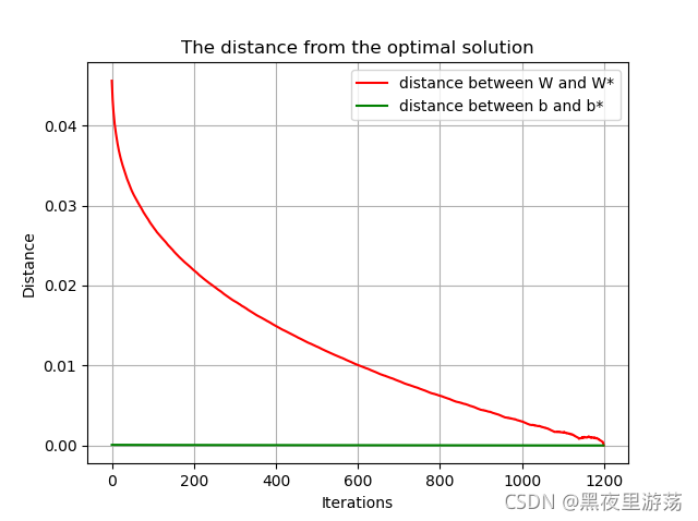
    # W和b距最优解的距离随迭代次数的变化
    plt.title('The distance from the optimal solution')
    plt.xlabel('Iterations')
    plt.ylabel('Distance')
    plt.plot(dis_W, 'r', label='distance between W and W*')
    plt.plot(dis_b, 'g', label='distance between b and b*')
    plt.legend()
    plt.grid()
    plt.show()

# ----------参数输入---------------
lr = 1e-5
batch_size = 10000
epochs_num = 20
# 运行函数
run(lr, batch_size, epochs_num)

lr = 1e-5 bs = 1000 epoch=20